
Many of us might have heard about “risk aversion“, which is a general dislike for risk. But, what is “ambiguity aversion”? To address this question, we need to first distinguish between “risky events” and “ambiguous events”. Let’s do that through a practical example.
Imagine a simple coin toss game where you win $1 if the coin lands on heads and lose $1 if it lands on tails. If the coin is fair, you know that you’ll win $1 with a 50% probability and lose $1 with a 50% probability. In this case, the probability distribution of outcomes is known, and you can quantify your expected return and risk. So, this game qualifies as a “risky event”.
What if you play the same game with a biased coin without knowing the probabilities of heads and tails? Now, the probabilities associated with the two possible outcomes are unknown. Therefore, you are in the dark about the degree of risk you’d be bearing if you played the game with such a coin. This is an example of an “ambiguous event”.
There is ample evidence that people are ambiguity averse such that they’d prefer to play the game with a fair coin rather than a biased coin with unknown probabilities, even though the bias could be substantially in their favor. This is also known as the ambiguity effect.
Table 1 below summarizes the comparison between risky events and ambiguous events. The idiom “better the devil you know than the devil you don’t” is often used to encapsulate the spirit of ambiguity aversion. In the rest of this lesson, we delve deeper to explain how the ambiguity effect can have an impact on our daily choices through real-world examples. We also discuss the Ellsberg paradox, which is based on experiments designed to demonstrate ambiguity aversion.
| Event type | Probability distribution of outcomes | Example |
|---|---|---|
| Risky event | Known | Fair coin toss: equal chances of heads vs. tails |
| Ambiguous event | Unknown | Biased coin toss with unknown probabilities of landing on heads vs. tails. |
Contents
Real-world examples of ambiguity aversion
Nonparticipation in capital markets
An influential paper by Easley and O’Hara (full reference here) investigates the implications of ambiguity aversion for stock markets and bond markets.
They start their paper by pointing out that, prior to the mid-1990s, more than two-thirds of American households held neither stocks nor bonds according to survey evidence. They go on to argue that this may be because some individuals find the ambiguity in capital markets too great and, thus, avoid investing in stocks or bonds. Their results indicate that regulations crafted with ambiguity aversion in mind can help increase participation in capital markets.
Healthcare treatments
A study by Berger et al. (2013) (full reference here) examines the implications of ambiguity aversion in the context of healthcare. They focus on ambiguity regarding:
- The diagnosis of a patient,
- The effects of treatment.
They find that the former case, which they label “diagnostic ambiguity”, results in an increase in the decision maker’s (i.e., the medical professional’s) propensity to opt for treatment. Conversely, there’s a reduction in the propensity to choose treatment in the latter case, which they refer to as “therapeutic ambiguity”.
Product reviews
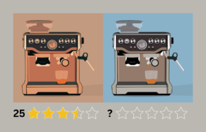
Imagine you’re interested in purchasing a new coffee machine. You’ve identified two models that have similar features and the same price: machine A and machine B. You decide to check product reviews to help with your decision. For machine A, you find lots of reviews, some positive and some negative. You judge that the machine is OK but not outstanding in any way. For machine B, despite searching for a long time, you can’t find even a single review.
Now, the question is the following: Assuming you don’t have any other choices and need to make a purchase, would you buy machine A or machine B? In this scenario, you can expect an ambiguity-averse individual to choose machine A as this machine is OK and would do the job. Of course, machine B could turn out to be superior to machine A, but because of the ambiguity, the individual leans towards machine A.
URL shorteners
Many of us have come across shortened URLs. For example, the full URL for our video tutorial on calculating the correlation coefficient between the returns of two stocks is as follows:
https://www.initialreturn.com/calculating-correlation-between-two-stocks/
And, here is a shortened URL for the same tutorial:
Both links would take you to the same page. But, which one would you prefer to click?
The first link shows both the domain name (initialreturn.com) and the title of the page (calculating the correlation between two stocks), whereas the second link is completely ambiguous about both aspects. Many people would prefer to click on the first link for that reason. As a separate note, always check the actual link address matches what’s shown on the link as scammers often use this tactic to take you to a different page.
Ellsberg paradox
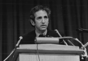
The paradox was put forward by the American economist Daniel Ellsberg in the 1960s (see the full reference here). It is based on a set of experiments he uses to motivate his arguments about ambiguity aversion.
The two-urns experiment
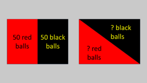
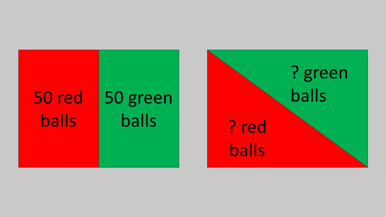
In this experiment, there are two urns. Both contain red balls and black balls. You are asked to choose one of these urns. Then, one ball will be drawn randomly from your chosen urn. If it’s a red ball, you’ll earn a big prize (say $100). If it’s a black ball you’ll earn a small prize (say $0 for simplicity). You’re given the following information about these urns:
- Urn 1: 100 balls in total, but the ratio of red balls to black balls is unknown.
- Urn 2: 50 red balls, 50 black balls.
In this case, most people prefer Urn 2, which involves a “risky proposition”, over Urn 1, which involves an “ambiguous proposition”.
The one-urn experiment
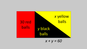
In this variation, there is a single urn that contains 90 balls in total. 30 of them red balls. The remaining 60 balls are either black or yellow, but in unknown proportions. In this case, which of the following two gambles would you prefer?
- Gamble 1: Draw a ball. You win $100 if it’s a red ball and nothing otherwise.
- Gamble 2: Draw a ball. You win $100 if it’s a black ball and nothing otherwise.
Many prefer Gamble 1 over Gamble 2. Note that the probability of drawing a red ball is 1/3. So, the choices made by decision-makers suggest that they believe there would be fewer black balls than yellow balls (although there’s no reason to expect that!), and, thus the probability of drawing a black ball is less than 1/3 according to their belief.
How about your choice between the following two gambles?
- Gamble 3: Draw a ball. You win $100 if it’s red or yellow and nothing if it’s black.
- Gamble 4: Draw a ball. You win $100 if it’s black or yellow and nothing if it’s red.
In this scenario, many prefer Gamble 4 over Gamble 3. However, this is inconsistent with preferring Gamble 1 over Gamble 2: Recall that choosing Gamble 1 over Gamble 2 implies a belief that the probability of drawing a black ball is less than 1/3. Such a belief suggests that the probability of winning Gamble 3 must be more than 2/3. But in that case, decision-makers should prefer Gamble 3 over Gamble 4 as the probability of winning Gamble 4 is 2/3. So, it seems (as in the previous experiment) that the ambiguity effect is at play here, such that individuals show a preference for the risky option (Gamble 4) over the ambiguous one (Gamble 3).
Summary
Ambiguity aversion can be summarized as our tendency to avoid options that have missing information. This stems from a general dislike of uncertainty or fear of the unknown. It is related to Frank Knight’s distinction between risk (measurable) and uncertainty (unmeasurable). It is distinct from risk aversion, such that risk aversion is about preferring a safe outcome over an expected outcome with the same value but with some risk. In contrast, ambiguity aversion involves giving more weight to “potential downsides” (or drawbacks) rather than “potential upsides” (or benefits) in ambiguous circumstances.
Further reading on ambiguity aversion:
Berger, Bleichrodt, and Eeckhoudt (2013) “Treatment decisions under ambiguity“, Journal of Health Economics, Vol. 32(3), pp. 559-569.
Easley and O’Hara (2009) “Ambiguity and Nonparticipation: The Role of Regulation“, The Review of Financial Studies, Vol. 22(5), pp. 1817–1843,
Ellsberg (1961) “Risk, Ambiguity, and the Savage Axioms“, The Quarterly Journal of Economics, Vol. 75(4), pp. 643–669.
what is next?
This lesson is part of our course on behavioral finance. If you’ve enjoyed this lesson, check out our other courses and tutorials as well. We’d always be happy to hear your thoughts about our content. You can reach us here. Last but not least, if you enjoy our content, don’t forget the spread the word to help us out!