
Descriptive statistics offer a simple way of understanding distributions of stock returns. They give us an idea about a distribution’s centrality, dispersion, symmetry, and other features. In this tutorial, we will show you how to generate descriptive statistics for stock returns using Excel’s data analysis tool.
Contents
Using Excel to get descriptive statistics for stock returns
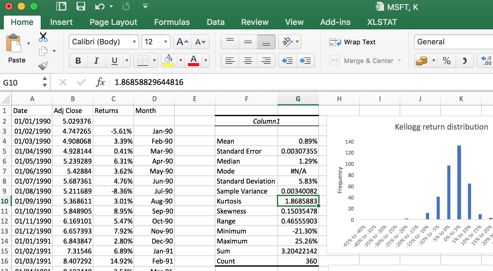
Once you’ve got the stock returns stored in a single column of an Excel spreadsheet, you can follow the steps below (see also Figure 1).
- If you haven’t used the data analysis tool in Excel before, make sure to enable the “Analysis ToolPak.”
- Then, go to the “Data” tab and click “Data Analysis.”
- In the menu that shows up, choose “Descriptive statistics” and hit the OK button.
- For the input range choose the column where the returns are recorded.
- If the first row is a label (e.g., stock ticker), tick the Labels in First Row box.
- Choose your output range (the results will be shown there).
- Tick the summary statistics box and click the OK button.

That’s it! At the end, you should see a table similar to Table 1 below.
| Mean | 0.020728949 |
| Standard Error | 0.004703466 |
| Median | 0.022081304 |
| Mode | #N/A |
| Standard Deviation | 0.089241997 |
| Sample Variance | 0.007964134 |
| Kurtosis | 2.208468759 |
| Skewness | 0.417298265 |
| Range | 0.751310035 |
| Minimum | -0.343529413 |
| Maximum | 0.407780621 |
| Sum | 7.462421559 |
| Count | 360 |
Mean return and median return
The statistics shown in Table 1 are based on the monthly returns of a stock over 30 years. So, there are 30 * 12 = 360 return observations in total as shown by the count.
The average return is given by the mean and is equal to 0.020728949, or 2.07%.
The median return is 2.21%. This means that 360 / 2 = 180 months yielded a return of less than 2.21% and the remaining 180 months yielded more than 2.21%.
Both the mean and the median inform us about the centrality of stock returns. In other words, they capture the average performance of the stock over the sample period.
The standard deviation of returns and variance of returns
First, let’s explain the relation between standard deviation and variance: Standard deviation is simply the square root of variance. Based on the data in Table 1, the variance is 0.007964134. Taking the square root yields √(0.007964134) = 0.089241997, which is indeed the standard deviation figure displayed in Table 1.
Both standard deviation and variance capture the dispersion of return observations around their mean. Specifically, a tight distribution around the mean would have a low standard deviation and variance. Conversely, if there were many returns observations far from the average, then the standard deviation and variance would both be high.
When computing the variance, we take the square of return observations, which makes it harder to interpret vis-à-vis the mean return. Since standard deviation is the square root of the variance, it can be more readily compared to the mean return. For example, based on the data in Table 1, we can say that the stock has an average return of 2.07% with a standard deviation of 8.92%. Therefore, standard deviation captures return volatility and is a measure of risk.
Skewness, kurtosis, and tails of a distribution
Skewness is about the symmetry of a distribution. For example, the normal distribution is symmetric around its mean. Symmetric distributions have a skewness of zero. It is common for stock return distributions to be asymmetric. A positive skewness implies a long tail to the right. This would imply a high occurrence of highly positive returns far from the average return. Conversely, a negative skewness suggests a long tail to the left. In this case, highly negative returns would be observed below the average return.
Kurtosis is all about the heaviness of the tails of a distribution. The normal distribution has a kurtosis of 3. For example, if a distribution has a kurtosis of 5, it is said to have an excess kurtosis of 5 − 3 = 2. Distributions that have positive excess kurtosis are considered to have fat tails (also known as leptokurtic distributions). This implies that extreme observations are more common in such distributions relative to otherwise similar normal distributions. Stock return distributions tend to be fat-tailed. Therefore, investors should be wary of the fact that they are likely to experience extreme return observations more often than they might like to believe.
Video tutorial
This video tutorial shows how to apply the steps above to obtain descriptive statistics for a specific stock in Excel.
Summary
In this tutorial, we illustrate how to use Excel’s “Descriptive statistics” analysis tool to obtain descriptive statistics for stock returns. Furthermore, we discuss mean return and median return as measures of centrality. Return volatility is captured by the standard deviations of returns. Finally, skewness is used to examine the symmetry of returns, and kurtosis is a useful statistic to analyze whether stock return distributions have fat tails.
What is next?
This tutorial is part of the series on analyzing stock returns.
- Next tutorial: The next tutorial explains how to compute the correlation between the returns of two stocks.
- Previous tutorial: We demonstrated how to plot a histogram of stock returns using Excel.
We hope you find these tutorials useful. Please share our content on social media to spread the word. If you would like to get in touch with us, you can do that through our contact page.