How to calculate Jensen’s alpha in Excel

The purpose of this tutorial is to teach you to calculate Jensen’s alpha in Excel. We’ll estimate the Jensen’s alpha on Amazon (AMZN) shares using the S&P500 as the market benchmark and the 13-week T-bill as the proxy of risk-free asset. Our analysis will be based on five years of monthly data (i.e., 60 observations in total).

Step 1: Compute excess returns

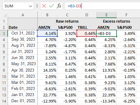
As you can see in Figure 1 below, we’ve entered the monthly raw returns on Amazon shares, the S&P500, and the treasury bill in columns B, C, and D, respectively. The first thing we need to do is to compute the excess returns on Amazon shares and the S&P500. This is simply achieved by subtracting the risk-free return as follows:

• Excess return on Amazon shares = Raw return on Amazon shares − Treasury bill return
• Excess return on S&P500 = Raw return on S&P500 − Treasury bill return

Step 2: Regress stock returns on market returns

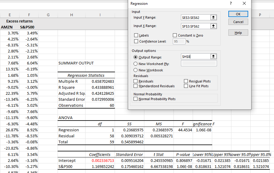
The second step is to regress the excess stock returns on the excess market returns. To do that, we’ll use Excel’s data analysis tool as follows:

1. If you haven’t used the data analysis tool in Excel before, make sure to enable the “Analysis ToolPak.”
2. Then, go to the “Data” tab and click on “Data Analysis.”
3. In the pop-up menu, choose “Regression” and click OK. This will bring up a new menu titled “Regression”.
4. For the Input Y range, select the excess stock returns (i.e., the excess Amazon returns in our example).
5. For the Input X range, choose excess market returns (i.e., the excess S&P500 returns).
6. Use the Output Range to specify where you want to see the regression output.
7. Click OK to run the regression.

These steps are illustrated in Figure 2 below.

Step 3: The Jensen’s alpha is the regression intercept

Once Excel provides the regression output, you need to find the Intercept as this is your Jensen’s alpha estimate. So, looking at the SUMMARY OUTPUT in Figure 2, we can see that Amazon’s α over the sample period was 0.002336713 or 0.23% per month (or 2.76% per annum).

We can also test the statistical significance of this estimate. We see that the t-statistic is very low (or the P-value is very high). Normally, we’d want to see a t-statistic higher than 1.64 (or P-value less than 0.1). Therefore, we can’t reject the null hypothesis that Amazon’s Jensen’s alpha is equal to zero. Intuitively, this suggests that we can’t confidently say that the stock’s α was different than zero over this period.

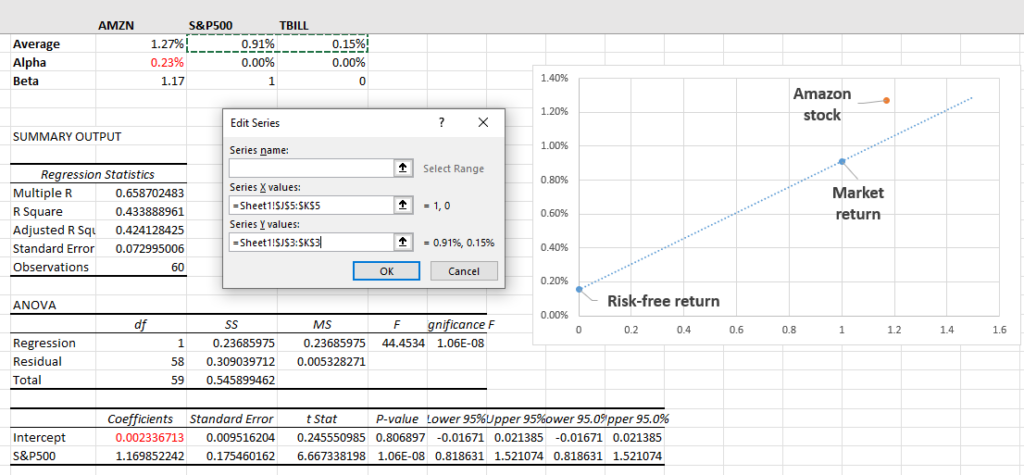
Step 4 (optional): Plot the security market line

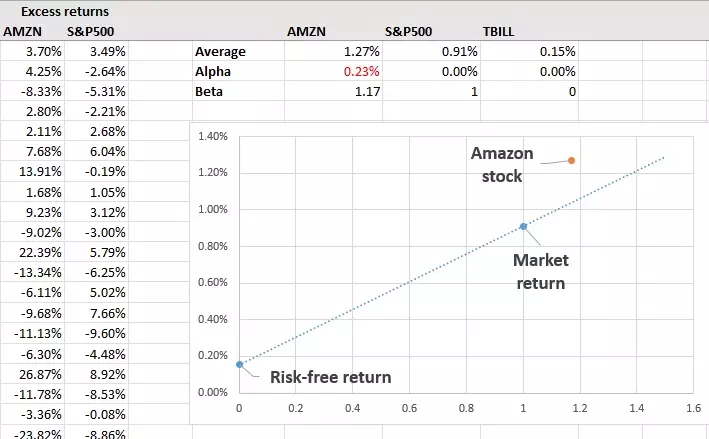
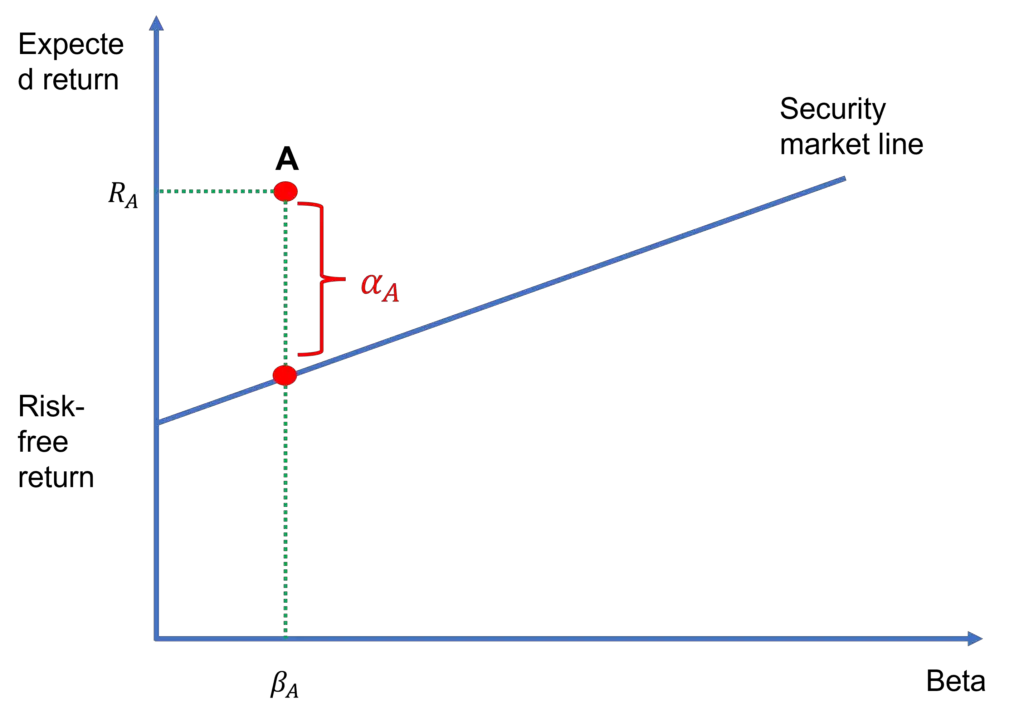
Finally, we can illustrate the Jensen’s alpha on a graph where the vertical axis represents the average return and the horizontal axis represents the beta.

We begin by plotting the security market line (SML). To do that, we need two data points:

• The first one is (S&P500 average return, S&P500 beta). By definition, the S&P500 beta is 1. And, the average return on the S&P500 was 0.91% per month during the sample period. So, we have (0.91%, 1).
• The second one is (T-bill average return, T-bill beta), Again, by definition, T-bill has a beta of 0. Its average return was 0.15% per month. Then, we have (0.15%, 0).

Next, we can insert a scatter plot in Excel to display these two points (see the blue points in Figure 3 below). After that, we add a trendline, which is the blue dotted line in Figure 3, to display the SML. Note that we format the trendline to include a forecast of 0.5 units. This extends the trendline beyond the market return (until β=1.5).

Finally, we add the Amazon stock as a separate data point to the chart (see the orange dot in Figure 3). We see that the Amazon stock lies above the SML. This is because it’s estimated alpha is positive. In fact, the alpha estimate of 0.23% is simply the vertical distance between the Amazon stock and the SML.

Video tutorial

Summary

Excel is extremely useful for investors in terms of conducting investment analysis. In this tutorial, we used Excel’s regression tool to regress excess returns on a stock on excess returns on a market index. We’ve interpreted the intercept of this regression as the stock’s Jensen’s alpha estimate. The regression output allows us to test the statistical significance of this estimate through the t-statistic (or the P-value) as well.

What is Next?

This tutorial is part of our series on analyzing stock returns.

• Previous tutorial: We explained how to calculate a portfolio’s risk and return in Excel.

If you enjoy following our tutorials, please support us by sharing our content with your friends and colleagues. If you’ve got any feedback for us, you can reach us here.