
In this tutorial, we’ll teach you how to calculate portfolio risk and return in Excel. We’ll focus on an example where we construct a portfolio of the following three stocks: Tesla (TSLA), Amazon (AMZN), and Netflix (NFLX).
If you’re unfamiliar with the formulas for portfolio return and portfolio risk, we’d recommend you check the following lessons first:
If you’re visiting this page from our YouTube channel, go to the “Video tutorial and Excel template” section below to download the Excel template used in that tutorial.
Contents
Step 1: Prepare the spreadsheet
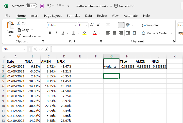
The first thing you need to do is to enter the returns of each stock in a separate column. As you can see in Figure 1 below, we’ve entered the dates in column A, and the returns on Tesla, Amazon, and Netflix in columns B, C, and D, respectively. Note that we’re working with monthly returns, but you can use any return frequency (daily, weekly, etc.) you like.
Feel free to check the following tutorials first if you’re unfamiliar with how to download stock price data and compute stock returns:
The next thing is to specify the investment weights for the portfolio. In this example, we’re assuming an equally-weighted portfolio such that we invest one-third of our funds in Tesla, one-third in Amazon, and the remaining one-third in Netflix. So, we’ve entered 1/3 (or 0.3333…) in cells H2, I2, and J2. Of course, you can choose any investment weight that you like.
Step 2: Use SUMPRODUCT & AVERAGE functions to compute portfolio return
We can now begin with computing the portfolio return. First, we need to use the AVERAGE function to compute the average realized returns for each stock. For instance, we enter:
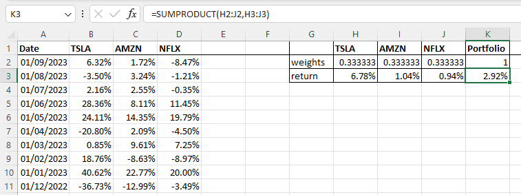
=AVERAGE(B2:B61)in cell H3 to get the average realized return for Tesla. This way, we find that the average returns of TSLA, AMZN, and NFLX are 6.78%, 1.04%, and 0.94%, respectively (see cells H3, I3, and J3 in Figure 2).
Next, we can use the SUMPRODUCT function to get the portfolio return (see cell K3 in Figure 2), since a portfolio’s return is simply the weighted average of the returns of each asset in that portfolio:
=SUMPRODUCT(H2:J2,H3:J3)
We find that the equally-weighted portfolio of Tesla, Amazon, and Netflix generated a return of 2.92% during our sample period.
Step 3: Use VAR.S and COVARIANCE.S functions to compute portfolio risk
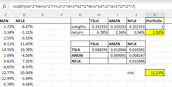
We can construct a variance-covariance matrix to calculate portfolio risk in Excel. This matrix includes both the variances of each stock and the covariances of each stock pair. All of these terms are part of the portfolio risk formula. We rely on the VAR.S function to compute the variances of each stock. For example, we enter:
=VAR.S(B2:B61)to get the variance of Tesla returns. Then, we use the COVARIANCE.S function to find the covariance between stock pairs. The covariance between Tesla and Amazon is calculated as:
=COVARIANCE.S(B2:B61,C2:C61)Finally, we use the portfolio risk formula to compute the risk of our portfolio as follows (see K10 in Figure 3 below):
=SQRT(H2^2*H6+I2^2*I7+J2^2*J8+2*H2*I2*I6+2*H2*J2*J6+2*I2*J2*J7)where H2, I2, and J2 are the investment weights; H6, I7, and J8 are variances; and I6, J6, and J7 are covariances. Note that we take the square root (using the SQRT function) to obtain the return volatility (i.e., the standard deviation of portfolio returns). If we didn’t, we’d be getting the variance of portfolio returns. We find that our portfolio has a return volatility of 12.23%.
A faster method
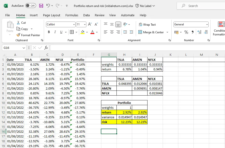
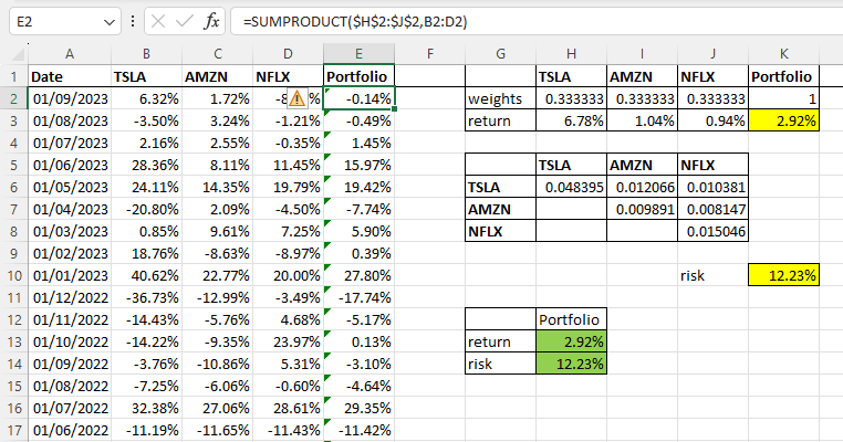
An alternative way of computing the risk and return of the equally-weighted portfolio of TSLA, AMZN, and NFLX is to add a new column that contains the monthly returns of this portfolio (see column E in Figure 4 below). For example, the portfolio’s return for August 2023 (i.e., from 01/08/2023 to 01/09/2023 in a day/month/year format) is calculated in cell E2 as:
=SUMPRODUCT($H$2:$J$2,B2:D2)Notice that we fix the cells of the first array because we’ll always use the same investment weights as we extend this formula downwards. Once we have all the monthly return observations in column E, we calculate portfolio return in cell H13 as:
=AVERAGE(E2:E61)And, portfolio risk in cell H14 as:
=STDEV.S(E2:E61)Note that we directly use the standard deviation function (STDEV.S) instead of computing the portfolio variance first and then taking its square root to obtain return volatility, which would have given the same result.
As you can see from Figure 4, the figures we get using the faster method (cells highlighted in green) match those obtained earlier (cells highlighted in yellow). The advantage of the current method is that it’s faster as we save time by not constructing the variance-covariance matrix.
Video tutorial and Excel template
Here is the Excel template we use in this video tutorial.
Summary
At the start of this tutorial, we explained how to use the AVERAGE and SUMPRODUCT functions in Excel to obtain the return of a portfolio. Then, we showed how the VAR.S and COVARIANCE.S functions can be used to construct a variance-covariance matrix, which can be employed to compute the portfolio’s return volatility. Finally, we demonstrated a faster method of obtaining portfolio risk in Excel without constructing the variance-covariance matrix.
What is Next?
This tutorial is part of our series on analyzing stock returns.
- Previous tutorial: We have explained how to estimate a stock’s beta in Excel.
If you enjoy our content, feel free to share our resources with others. And, we’d love to hear any feedback you’ve got for us. You can reach us here.