How to calculate beta in Excel

In this tutorial, we’ll show you how to calculate beta in Excel. First, we explain the data you need before getting started. Then, we offer four different ways of computing betas in Excel (the first one is the fastest if you’re in a rush!). If you prefer a video tutorial, that is provided at the end as well.

What you need for estimating betas

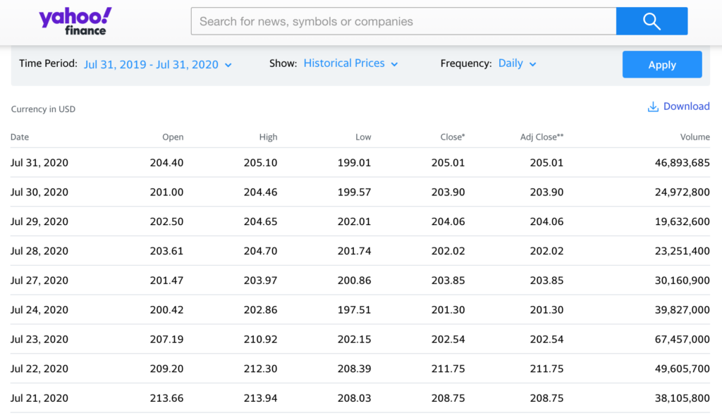
Let’s assume that you’d like to compute the beta of a particular stock, say, Tesla ($TSLA) using S&P500 as the benchmark index. Then, you need the first decide on your sample period. A common choice is monthly returns over a 5-year period, but you can consider alternatives (e.g., daily returns over the past year) as well. Once your sample period and data frequency are determined, you need to obtain:

• Returns on the security you’re interested in (Tesla in our example).
• Returns on a market index (S&P500 in our example).

If you need to calculate beta using excess returns, in addition to the data on raw returns mentioned above, you need to download returns on a treasury bill (T-bill) to serve as a proxy of the risk-free rate. Then, for each period, you can obtain the excess return by subtracting the T-bill return from the raw return.

Different ways of computing beta in Excel

After obtaining your data, you can use any of the methods described below to compute beta.

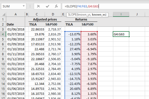
Method 1: Slope function

This is the quickest method and works as follows:

1. Choose an empty cell and enter =slope to trigger Excel’s slope function.
2. For known_ys, choose the returns on the security you’re interested in.
3. For known_xs, choose market returns.
4. Hit the enter button to obtain the beta.

See Figure 1 below for an illustration of these steps.

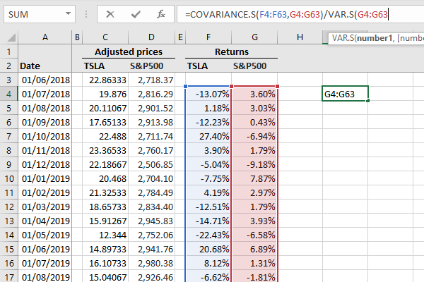
Method 2: Covariance and variance functions

Mathematically, a security’s beta β_i is equal to the covariance between the returns of that security and the market σ_im divided by the variance of market returns σ_m² (see also our lesson on CAPM):

Then, we can obtain the beta using this formula as follows:

1. Choose an empty cell and enter =covariance.s to use Excel’s covariance function.
2. For array1, choose the returns on the security you’re interested in.
3. For array2, choose market returns.
4. Then, type the division symbol / in the same cell.
5. Next, type var.s to use the variance function.
6. In the number1 field of this function, select market returns.
7. Finally, press enter to get your beta estimate.

These steps are summarized in Figure 2.

Method 3: Linear regression

The third method is based on regressing the security’s returns on the market returns to obtain the beta as follows:

1. If you haven’t used the data analysis tool in Excel before, make sure to enable the “Analysis ToolPak.”
2. Then, go to the “Data” tab and click on “Data Analysis.”
3. In the pop-up menu, choose “Regression” and click OK. This’ll bring up a new menu titled “Regression”.
4. For Input Y range, select the security’s returns.
5. For Input X range, choose market returns.
6. Use the Output Range to specify where you want to see the regression output.
7. Click OK to run the regression.
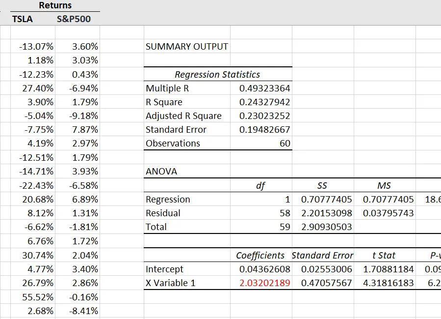
8. In the summary output that is displayed in your worksheet, look at the final row. Your beta estimate is the coefficient on the market returns (your X variable).

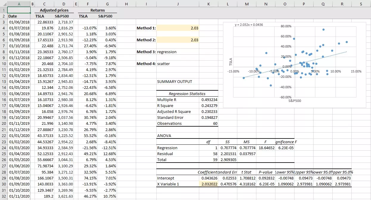
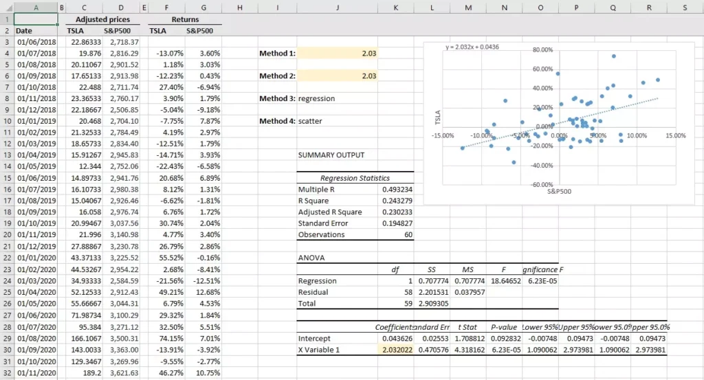
Figure 3 shows the summary output you’d get after regressing the security’s returns on market returns. The figure in red is the beta estimate based on this linear regression.

Method 4: Scatterplot and trend line

The final method involves producing a scatter diagram of the security’s returns against market returns.

1. Go to the “Insert” tab and click on the “Insert Scatter (X, Y) or Bubble Chart” icon. This should bring an empty chart. Make sure you keep it selected.
2. Find the “Chart Design” tab and click “Select Data”.
3. In the pop-up menu that comes up, click “Add” under “Legend Entries (Series)”, which should bring up a new menu.
4. For the Series X values, enter the range of market returns.
5. For the Series Y values, enter the range of returns on the security you’re interested in.
6. Click OK, and OK again. This should produce the chart.
7. Once the chart is produced, make sure it’s selected, and click “Add Chart Element” under the “Chart Design” tab.
8. In the dropdown menu, go to “Trendline” and choose “Linear”. This should add the trendline to the chart.
9. Lastly, repeat the previous step, but click “More trendline options” at the end.
10. In the “Format Trendline” panel that appears on the right, check the “Display Equation on chart” option.
11. Once you do that, an equation that looks like this will appear on the chart: y = 2.032 x + 0.0436. In this case, the beta estimate is 2.032, which is the slope of the trendline (and that’s why Method 1 uses the slope function).

In Figure 4, you can see the equation of the trendline (or the linear regression line) in the top-left corner of the scatterplot.

Video tutorial: Calculating beta in Excel

What is next?

This tutorial on how to calculate beta in Excel is part of our series on analyzing stock returns.

• Next tutorial: We’ll show how to use functions in Excel to compute a portfolio’s risk and return.
• Previous tutorial: We showed how Excel can be used to calculate the correlation between two stocks.

If you enjoy our content, feel free to spread the word by sharing our posts with your friends and colleagues. And, we’d be happy to hear back from you if you’ve got any questions or suggestions. Here is our contact page.