
The capital asset pricing model (or CAPM) is among the most widely-used asset pricing models by stock analysts and portfolio managers. Its popularity arises from its simplicity and elegance. Analysts and investors can use it to forecast returns or to estimate the cost of equity. In this lesson, we explain this model and its assumptions. We provide an easy-to-use calculator as well.
Contents
CAPM calculator

You need the following inputs to use the CAPM calculator:
- The beta of the asset. This can be estimated based on historical returns.
- The risk-free rate of return. This is often proxied by the yield on a selected government bond.
- Expected return on the market portfolio. Historical returns on a market index such as S&P500 can be a starting point, with the analyst adjusting this based on his beliefs about future performance.
Example: If a stock’s beta is 1.2, the risk-free rate is 3%, and the expected market return is 8%, you can verify using the calculator above that the stock’s expected return is 9%.
CAPM equation
CAPM equation can be stated as follows:

This equation suggests that a stock’s (or any risky asset’s) expected return E[Ri] depends on its beta βi, the riskless rate of return Rf, and the market’s expected return E[Rm]. More specifically, it states that:
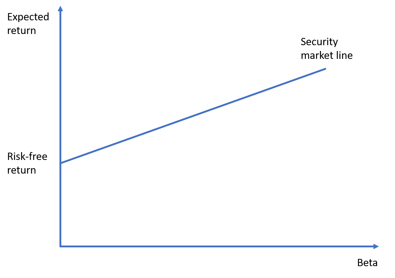
Expected return = Risk-free rate + Risk premium
where the risk premium βi (E[Rm] − Rf) is higher for stocks with higher betas. This is because beta is a measure of systematic risk, and high-beta stocks bear more systematic risk compared to low-beta ones.
It is worth noting that the CAPM equation applies to portfolios of assets (think of investment funds) as well as individual assets.
CAPM assumptions

We can list the CAPM assumptions as follows:
- Investors act rationally and are mean-variance optimizers.
- They are assumed to agree on the expected return and variance of each asset and covariances between asset pairs. This means that they will all end up with the same optimal risky portfolio when they engage in mean-variance optimization.
- They have a single investment period (e.g., a year) in mind.
- All assets are tradeable and perfectly divisible.
- Investors are price takers (i.e., their trades do not influence prices).
- They can lend or borrow unlimited amounts at a common risk-free rate.
- Short selling is allowed without limits.
- There are no taxes and transaction costs (e.g., trading commissions).
Note that these are the assumptions for the standard version of the model. Extended versions of the model relax some of these assumptions. For example, one of the extensions allows for differential rates for borrowing and lending.
Summary
The capital asset pricing model concerns itself with the pricing of risky assets in market equilibrium. It posits that if all investors engage in mean-variance optimization in the spirit of modern portfolio theory, the optimal risky portfolio becomes the market portfolio. And, because idiosyncratic risk is diversified away within the market portfolio, investors require a risk premium on market risk only, which is captured by beta. As a result, CAPM predicts a linear relationship between an asset’s expected return and its beta.
The model dates back to the 1960s and is based on separate works by William Sharpe, Jack Treynor, John Lintner, and Jan Mossin.
Further reading:
Sharpe (1964) ‘Capital Asset Prices: A Theory of Market Equilibrium under Conditions of Risk‘, The Journal of Finance, Vol. 19 (3), 425-442.
What is next?
If you’ve enjoyed reading this post, we’d recommend you check our investments course, which is accessible for free.
- Next lesson: We will focus on the security market line, which is a visual illustration of the CAPM equation.
- Previous lesson: We explained the distinction between systematic risk and idiosyncratic risk.
As a final word, if you like reading our content, you can support us by spreading the word! So, feel free to share our posts with your friends and colleagues.