
In previous lessons, we explained that when there is no risk-free asset in an economy, investors should invest in one of the portfolios that lie on the efficient frontier based on their risk tolerances. But, if a risk-free asset exists, then there is a unique portfolio that all investors should invest in. In particular, the optimal risky portfolio is the unique portfolio that is tangent to the efficient frontier when combined with the risk-free asset. According to the modern portfolio theory, the best option for an investor is to split their funds between the optimal risky portfolio and the risk-free asset.
In this lesson, we will teach how to locate the optimal risky portfolio on the efficient frontier from both a theoretical perspective and a practical one using Excel. You can watch our video tutorial and download the Excel spreadsheet as well.
Contents
Locating the optimal risky portfolio
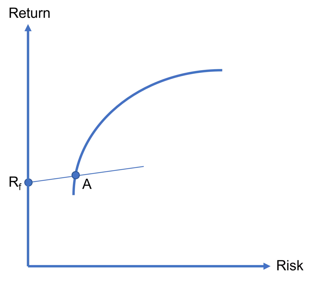
In the previous lesson, we explained that the combinations of a risky asset and the risk-free asset are represented as a straight line in the risk-return space, which is known as a capital allocation line.
If investors can combine the risk-free asset with any risky asset, it makes sense for them to focus on risky assets that lie on the efficient frontier as those assets (known as efficient portfolios) offer the best risk-return tradeoff in the market. This is shown in Figure 1 where an investor is splitting her funds between the efficient portfolio A and the risk-free asset, which yields Rf.
There is an infinite number of efficient portfolios that lie on the efficient frontier, which raises the following question: Is portfolio A the best choice for our investor? The answer is no. She can do better, for example, by investing in portfolio B as discussed below.
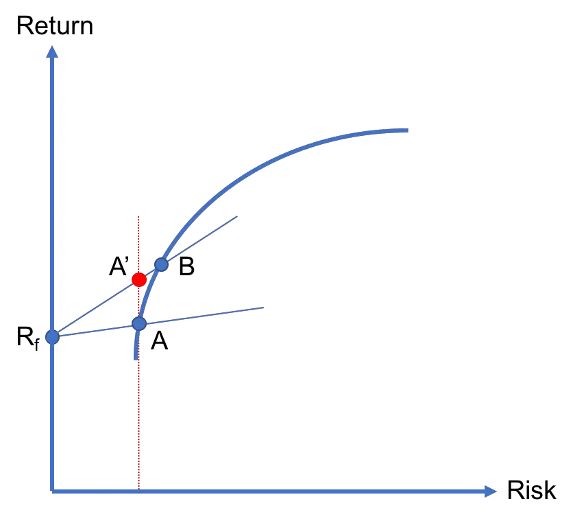
As shown in Figure 2, B is further up on the efficient frontier as compared to A. As a result, the capital allocation line that connects Rf and B lies above the one that connects Rf and A.
This has an important implication. Look at portfolio A’. It is a combination of the risk-free asset and B and lies directly above A. So, A and A’ have the same level of risk, but the latter offers a higher return. Thus, the investor would prefer A’ over A. In fact, for any combination of Rf and A, we can find a combination of Rf and B with the same risk but a higher return. As a result, the investor is better off splitting her wealth between Rf and B instead of Rf and A.
Could the investor still do better? Yes, she can! The investor has to seek the efficient portfolio that is the furthest along the efficient frontier and that can still be combined with the Rf. This is equivalent to maximizing the slope of the capital allocation line that goes through the risk-free asset and the efficient frontier.
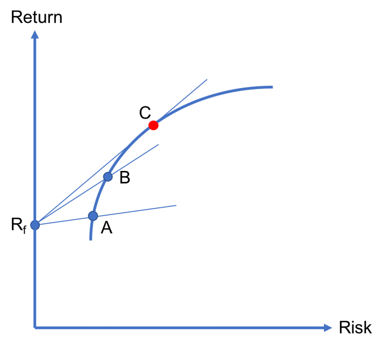
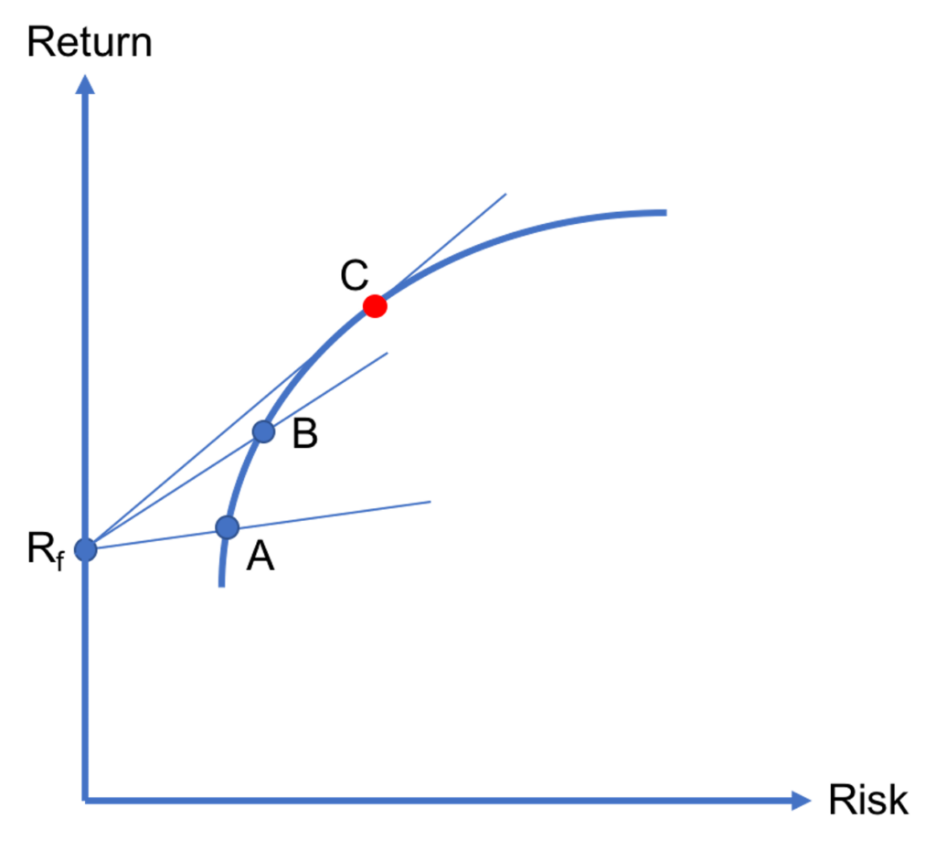
We illustrate this in Figure 3. As discussed earlier, B is better than A, since the capital allocation line involving the former has a steeper slope. By the same logic, C must be better than B, because it leads to a capital allocation line that has an even steeper slope. Furthermore, the capital allocation line that connects Rf and C is tangent to the efficient frontier. This means that it is impossible to combine Rf with any other efficient portfolio that lies further along the efficient frontier than C. Thus, this is the point where the slope of the capital allocation line is maximized. And, C is the optimal risky portfolio!
Using Excel to find the optimal risky portfolio
It is easy to find the optimal risky portfolio using Excel or other software. In the case of Excel, you will need to use the Solver add-in. If you haven’t used that before, you can enable it by going to File > Options > Add-ins. Once you are at the Add-ins tab, click the Go button where it says “Manage Excel Add-ins”. In the menu that pops up, simply check the “Solver Add-in” and hit the OK button. Once you’ve done that, you can go to the “Data” tab. And, you will find the Solver icon there.
To find the optimal risky portfolio, you need:
- The return and variance of each security you are examining.
- The covariance (or correlation) between each pair of securities.
- The risk-free rate of return.
Maximizing the Sharpe ratio using Solver
Looking at Figure 3 again, we see that the capital allocation line that goes through the optimal risky portfolio C has the steepest slope compared to other efficient portfolios such as A or B. In fact, the slope of that capital allocation line can be interpreted as the Sharpe ratio of C:

where RC is the return of the optimal risky portfolio C and σC is the return volatility of the same portfolio, which is a measure of portfolio risk. So, you need to use the Solver to maximize this Sharpe ratio. If you click the Solver button, pay attention to the following fields in the menu that pops up:
- Set objective: Assign this to the cell where you compute the Sharpe ratio using the equation above.
- By Changing Variable Cells: These are the cells that will contain the investment weights for each security.
- Subject to the Constraints: You should create a cell where you sum up the investment weights. Then, you should add a constraint that sets the value of this cell equal to 1.
In summary, your objective is to maximize the Sharpe ratio by changing the investment weights of the assets you are examining with the constraint that investment weights add up to 100%.
Video tutorial and Excel template
Summary
According to modern portfolio theory, investors engage in mean-variance optimization to find the efficient frontier. The portfolios that lie on the efficient frontier offer the best risk-return tradeoff in the market.
In this lesson, we have shown that when there is a risk-free asset in the market, there is a unique optimal risky portfolio. Then, investors’ remaining task is to simply decide how to split their funds between the risk-free asset and the optimal risky portfolio. Their decision will be driven by their risk preferences such that more (less) risk-averse investors would invest a higher (lower) proportion of their money in the risk-free asset.
Further reading:
Kan and Zhou (2007), “Optimal Portfolio Choice with Parameter Uncertainty“, Journal of Financial and Quantitative Analysis, Vol. 42 (3), pp. 621-656.
What is next?
This lesson is part of our course on investments.
- Next lesson: We will introduce the market portfolio as a value-weighted portfolio of all risky assets.
- Previous lesson: We explained that the capital allocation line represents combinations of a risky asset with the risk-free asset within a portfolio.
Please feel free to share this post within your network if you have enjoyed reading it. If you have any questions or would like to make some suggestions, you can fill out our contact form to reach us.