
When a risk-free asset exists in an economy, investors can add that asset to their portfolios if they wish so. In the risk-return space, the combination of the risk-free asset and any risky asset is a straight line. This line is called the capital allocation line as it shows how an investor’s capital is allocated between the risk-free asset and the risky asset.
Contents
Capital allocation line formula
The capital allocation line formula can be written as follows:

This is based on a two-asset portfolio that contains a risky asset A and the risk-free asset, such that μA is the return on asset A, σA is the return volatility for asset A, and Rf is the risk-free rate of return. And, μP and σP are the return and risk of this two-asset portfolio, respectively.
It is easy to notice that this formula fits the general equation for a straight line, which is:
y = mx + c
where m is the slope of the line and c is the intercept. Therefore, the slope of the capital allocation line is (μA − Rf) / σA and its intercept is Rf (i.e., the risk-free rate of return).
For those who are interested, the derivation of this formula is as follows. We begin with the general formulas of portfolio return and portfolio risk for a two-asset portfolio:

We let the first asset be our risky asset A and the second asset be the risk-free asset. In this case, we can rewrite the portfolio return as follows:
μP = ωA μA + (1 − ωA) Rf
Moreover, the portfolio risk simplifies into:
σP = ωA σA
This is because the return volatility of the risk-free asset is zero (i.e., σ2 = 0). Finally, if we plug ωA = σP / σA into the portfolio return equation, we obtain the equation presented at the beginning of this section.
Plotting the capital allocation line
Suppose that an investor has $1,000 to invest. She decides to split her funds between the risk-free asset Rf and an efficient portfolio A. In Figure 1, this is represented as the CAL that goes through Rf and A.
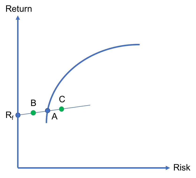
For example, if the investor invests $500 in Rf and $500 in A, her portfolio lies at point B, which is exactly halfway between Rf and A. If she invests $200 in Rf and $800 in A, her portfolio is still in between Rf and A but is closer to the latter as her portfolio is now 80% invested in A. Finally, if the investor borrows, say, $600 at the risk-free rate to invest $1,000 + $600 = $1,600 in A, her portfolio lies at point C, which is located to the right of A.
In summary, if the investor lends at the risk-free rate and invests in A, her portfolio would be located between Rf and A. But, if she borrows at the risk-free rate to invest more in A, then her portfolio would lie on the CAL to the right of A
CAL vs CML
Students sometimes wonder whether the CAL and the CML are the same things. The short answer is no. We can explain the difference as follows.
The capital allocation line depicts possible combinations of the risk-free asset with any risky asset (e.g., a particular stock) within a portfolio. In contrast, the capital market line shows possible combinations of the risk-free asset with the market portfolio in particular.
In that sense, CML is a specific case of CAL where the risky asset chosen is the market portfolio. According to the capital asset pricing model, CML offers the best tradeoff between expected return and volatility in the market. In fact, this is often referred to as the two-fund separation theorem whereby investors hold a combination of the market portfolio and the risk-free asset.
Summary
In this lesson, we explained that when a risky asset is combined with a risk-free asset, those portfolio combinations are represented by a straight line in the risk-return space and that straight line is known as the capital allocation line. We have derived its formula and have explained how it differs from the CML as well.
Further reading:
Markowitz (1991), “Foundations of Portfolio Theory“, Journal of Finance, Vol. 46 (2), pp. 469-477.
What is next?
This lesson is part of our course on investments.
- Next lesson: We will explain how mean-variance optimizers can locate the optimal risky portfolio in a market with a riskless asset.
- Previous lesson: We showed how to obtain the minimum-variance portfolio, which is the efficient portfolio with the lowest risk.
We always appreciate feedback from our visitors. If you notice any errors in content or if you have any questions or suggestions for us, you can write to us here.